Flow Differential Equations
I am interested in developing simple 2D erosion models to simulate, for purely visual purposes, plant leaf vein formation. There is a "canalization hypothesis" for vein formation whereby pathways for auxins in young leaves are self-reinforcing. These pathways eventually become the veins in mature leaves. I am no botanist, but it seems plausible that a self-reinforcing process can yield the tree-like structure of a leaf, since waterways erode away a landscape in a (somewhat) similar branching fashion.
Intro
After substantial trial-and-error not worthy of recapitulation, I wish to investigate the following model: \[ \begin{align*} h&:W \to \mathbb{R} \text{ an elevation map} \\ f &= -\frac{\nabla h}{\|\nabla h\|} \\ G(U) &= \mu\left(\left\{\mathbf{x}\in W : \text{a streamline of }f\text{ originating at }\mathbf{x}\text{ passes through }U \right\} \right)\,, \end{align*} \] A few notes:
- A "streamline of \(f\) originating at \(\mathbf{x}\)" is defined as a \(C^1\) solution \( \gamma:[0,a) \to W \) to the differential equation \(\gamma'(t)=f(\gamma(t))\) with \(\gamma(0)=\mathbf{x}\). Streamlines are not unique in general; consider that \(f(x,y)=(1,y^{1/3})\) has streamlines \(\gamma_1(t)=(t,0)\) and \(\gamma_2(t)=(t,\sqrt{\frac{8}{27}}t^{3/2})\) both passing through the origin.
- \(W\) is a bounded, open set. It is bounded so that it has finite Lebesgue measure, and open so that we don't have to do legwork to define \(\nabla h\) on all of \(W\).
- \(h\) must not have any local extrema in \(W\) to avoid division by zero in \(f\).
- Typically, normalizing \(f\) does not change any streamline. If \(\gamma\) is some streamline of \(f\) and \(\alpha:[0,a)\to \mathbb{R}\) monotone increasing, then \((\gamma\circ \alpha)'(t)=\gamma'(\alpha(t))\alpha'(t)=f((\gamma\circ\alpha)(t))\alpha'(t)\). The differential equation \(\alpha'=g\circ\gamma\circ\alpha\) has a solution on \([0,a)\) for sufficiently nice \(g\) and \(\gamma\), so we can construct a coincident streamline for \(fg\). At any rate, we explicitly don't want to deal with the situation where water is going infinitely slow and never makes it to the bottom of the hill. Normalization is a good way to avoid it.
- \(\mu\) is the ordinary Lebesgue measure. For our purposes, we might as well define \(G\) to take the measure of the interior of the set of streamline origins. This would make it very clear that our sets are measurable. But we won't be dealing with non-measurable \(U\) and won't be invoking the axiom of choice anywhere, so I won't bother.
Streamline Existence and Uniqueness
Picard iterates are the typical approach to existence and uniqueness questions regarding streamline-like ODEs. Consider the equation \(\gamma'(t)=(f\circ \gamma)(t)\) in a neighborhood \(U\) of the origin, for \(t\in [-\epsilon, \epsilon]\). Without loss of generality, by translation and rotation, assume that \(\gamma(0)=0\) and \(f(0)=\gamma'(0)=(1,0)\). The Picard iteration of a function \(\gamma_k:[-\epsilon, \epsilon]\to U\) is the application of an operator \(T\) so that \[\gamma_{k+1}(t)=T(\gamma_k)(t)=\int_0^t (f\circ \gamma_k)(s)\, ds\,. \] The idea is to show that \(T\) is a contraction mapping, and use the Banach fixed point theorem to construct the unique fixed point \(\gamma\) of \(T\). Since \(\gamma(t)=\int_0^t (f\circ \gamma)(s)\,ds \iff \gamma'(t)=(f\circ \gamma)(t)\) when \(f\) is continuous, this shows that there is a unique streamline passing though the origin.
Part of our goal here is to classify uniqueness of streamlines based on local properties of \(f\). We've already supposed that \(f\) is continuous. More is needed, however, for uniqueness.
Note: Let real-valued \(g\) be Lipschitz in a neighborhood \(U\) of zero, and \(h\) differentiable with bounded derivative in \(g(U)\). Then for \(x,y\in U\), \[ |h(g(x))-h(g(y))| \leq |g(x)-g(y)|\sup_{z\in g(U)}|h'(z)|\,, \] showing that \(h\circ g\) is also Lipschitz in \(U\). Applied to \(|f_x(\mathbf{p})|=\sqrt{1-f_y(\mathbf{p})^2}\), we see that \(f_x\) is Lipschitz if \(f_y\) is Lipschitz and contained in, say \([-1/2,1/2]\). Since \(f_y\) is continuous, it is not a problem to enforce the range of \(f_y\) by shrinking \(\epsilon\) as needed. For this reason, we may assume that \(f_x\) is Lipschitz as well.
Proof. There is an straight-forward reduction from this ostensibly 2D case to a 1D ODE. Suppose we find a solution \(\gamma\) in the neighborhood of the origin. Let \(F(x,t,y)=\gamma(t)-(x,y)\) so that the projection of \(\{F(x,t,y)=0\}\) is the image of \(\gamma\) and \[ DF(x,t,y)=\begin{bmatrix}-1&\gamma_x'(t)&0\\0&\gamma_y'(t)&1 \end{bmatrix}\,. \] Since \(f\) is continuous, there is a neighborhood of the origin where \(f_x\) is positive and bounded away from zero. Here \(\gamma_x'(t)\) is strictly positive and the submatrix \(\begin{bmatrix}\gamma_x'(t)&0\\ \gamma_y'(t)&1 \end{bmatrix}\) invertible. By the implicit function theorem, \(\{F(x,t,y)=0\}\) is the graph of a \(C^1\) function \(g(x)\). Simply omitting the \(t\) component in the output of \(g\) yields a \(C^1\) function (which we will still call \(g\)) with graph equal to the graph of \(\gamma\) in this neighborhood. Moreover, \[(1,g'(x))=\frac{\gamma_y'(t(x))}{\gamma_x'(t(x))}=\frac{f_y(x, g(x))}{f_x'(x,g(x))}\implies g'(x)= \frac{f_y(x,g(x))}{f_x(x,g(x))}\,. \] On the other hand, suppose we find a solution \(g\) for the ODE \[g'(x)= (f_y/f_x)(x,g(x))\] in the neighborhood of the origin. Then set \(\gamma\) to be the arc-length parameterized version of \(\tilde{\gamma}(t)=(t,g(t))\). We find that, for \(\gamma(t)=(\tilde{\gamma}\circ \alpha)(t)\), \[ \begin{align} \gamma'(t) &= (\alpha'(t), g'(\alpha(t))\alpha'(t)) \\ &= \alpha'(t) (1, (f_y/f_x)(\alpha(t), g(\alpha(t)))) \\ &= \alpha'(t) (f_x(\alpha(t), g(\alpha(t))), f_y(\alpha(t), g(\alpha(t)))) \\ &= f(\alpha(t), g(\alpha(t))) \\ &= f(\gamma(t))\,. \end{align} \] Line (4) follows from (3) since both \(\gamma'\) and \(f\) have unit length.
Both of these maps (one taking a \(\gamma\) to a \(g\) and the other taking a \(g\) to a \(\gamma\)) are injective, so we've constructed a bijection between solutions \(\gamma\) and solutions for the ODE \(g'(x)= (f_y/f_x)(x,g(x))\). We will show existence and uniqueness for the latter ODE. For convenience we'll denote \(f_y/f_x\) as \(\tilde{f}\). Since \(f_x\) is continuous and bounded away from zero in a neighborhood of the origin, \(\tilde{f}\) is continuous on that same neighborhood. Likewise, since both \(f_x\) and \(f_x\) are Lipschitz in a neighborhood of the origin, with \(f_x\) bounded away from zero, \(\tilde{f}\) is also Lipschitz.
We're going to be working in a subspace of \(C^1([-\epsilon, \epsilon])\), the space of continuously differentiable functions from the interval \([-\epsilon,\epsilon]\) to \(\mathbb{R}\). It is well-known that with the norm \[ \|g\|_{C^1}:=\sup_{x\in[-\epsilon,\epsilon]}\left| g(x)\right|+\sup_{x\in[-\epsilon,\epsilon]}\left|g'(x)\right|\,, \] \(C^1([-\epsilon,\epsilon])\) is a Banach space. Now consider the subset \[ C^1_0([-\epsilon, \epsilon]):=\{g\in C^1([-\epsilon,\epsilon]) : g(0)=0\}\,. \] Since \( C^1 \) convergence implies point-wise convergence, any sequence \((g_n)_n\subset C^1_0([-\epsilon,\epsilon])\) converging (in \(C^1([-\epsilon,\epsilon])\)) to \(g\) has \(g(0)=0\); this shows that \(C^1_0([-\epsilon,\epsilon])\) is closed as a subset of \(C^1([-\epsilon,\epsilon])\), and indeed a Banach space itself.
Moreover, for \(g\in C^1_0([-\epsilon,\epsilon])\) and \(x\in [-\epsilon,\epsilon]\), \[\begin{align*} \left|g(x)\right| &= \left|g(0)+\int_0^x g'(x)\,dx\right| \\ &\leq 0+\int_{[\min(0,x),\max(0,x)]} |g'(x)| \, dx \\ &\leq \epsilon \sup_{x\in [-\epsilon, \epsilon]} |g'(x)| \end{align*}\] so that \[\sup_{x\in[-\epsilon,\epsilon]} |g'(x)|\leq\left|g\right|_{C^1}\leq (1+\epsilon)\sup_{x\in[-\epsilon,\epsilon]} |g'(x)|\,.\] Since these metrics are equivalent for \(C^1_0\), we'll use the simpler version \(\|g\|_{C^1_0}=\sup_{x\in[-\epsilon,\epsilon]} |g'(x)|\).
Since \(\tilde{f}\) is continuous, the fundamental theorem of calculus asserts that the Picard operator \(T\) defined by \[T(g)(x):=\int_0^x (\tilde{f}\circ g)(s)\,ds\] is a map \(C^1_0([-\epsilon,\epsilon])\to C^1_0([-\epsilon,\epsilon])\), and indeed \[ \begin{align*} \|T(g_1)-T(g_2)\|_{C^1_0}&=\sup_{x\in [-\epsilon,\epsilon]} \left| \frac{d}{dx}\left(\int_0^x (\tilde{f}\circ g_1)(s)\,ds - \int_0^x (\tilde{f}\circ g_2)(s)\,ds\right) \right| \\ &= \sup_{x\in [-\epsilon,\epsilon]} \left|(\tilde{f}\circ g_1)(x)-(\tilde{f}\circ g_2)(x) \right|\,. \end{align*} \] To show that \(T\) is a contraction mapping, we'll have to compare this to \[ \|g_1-g_2\|_{C^1_0}=\sup_{x\in[-\epsilon,\epsilon]}\left|g_1'(x)-g_2'(x)\right|\,. \] If \(\tilde{f}\) has Lipschitz constant \(k\) in \([-\epsilon, \epsilon]\), then \[\begin{align*} \left|(\tilde{f}\circ g_1)(x)-(\tilde{f}\circ g_2)(x)\right|& \leq k|g_1(x)-g_2(x)| \\ &\leq k\left|\int_0^x (g_1-g_2)'(x)\,dx \right| \\ &\leq k\epsilon \|g_1-g_2\|_{C^1_0}\,. \end{align*}\] Here \(k\) is a constant for \(\tilde{f}\), so by choosing \(\epsilon < 1/k \), we have found that \(T\) is a contraction mapping. The Banach fixed point theorem asserts the unique fixed point \(g\) of \(T\), so that \(g'(x)=(\tilde{f}\circ g)(x)\). This completes the proof. (QED)
More can be said here; not all vector fields \(f\) failing the \(f_y\) Lipschitz condition yield multiple solutions for \(\gamma'=f\circ \gamma\). As much as I'd like to dwell on further delineation of the boundary between "unique solution" and "multiple solutions," the truth is that from a computational standpoint everything is Lipschitz; so I should keep moving and be aware of increasing convergence time when \(f\) becomes "less" Lipschitz.
To round out our discussion on streamlines, we show how to extend Picard's theorem to entire streamlines.
Proof. Let \(Y\) be all points \(y\in W\) so that there is a differentiable \(\gamma_y:(a_y,b_y)\to W\) with \(\gamma_y(0)=\mathbf{x}_0\), \(\gamma_y(t)=y\) for some \(t\in (a_y,b_y)\), and \(\gamma_y'=f\circ \gamma_y\). Define a function \(\eta:Y\to \mathbb{R}\) by \(\eta(y):=\gamma_y^{-1}(y)\), and set \(\gamma:\eta(Y)\to Y\) equal to \(\eta^{-1}\). The claim is that \(\gamma\) is a maximal solution to \(\gamma(0)=\mathbf{x}_0, \gamma'=f\circ \gamma\) in W, in the sense that any other solution is a restriction of \(\gamma\).
The core lemma here is the following: let \(\gamma:(a,b)\to W\) and \(\lambda:(a,b)\to W\) satisfy our flow differential equation \(\gamma'=f\circ\gamma\) with \(\gamma(0)=\lambda(0)=\mathbf{x}_0\). Then \(\gamma\) and \(\lambda\) are the same function. If not, say WLOG for some \(t>0\), then for \(c:=\inf\{t>0:\gamma(t)\neq \lambda(t)\}\) finite we have:
- \(\gamma(c)=\lambda(c)\) since both are continuous
- \(\gamma\) and \(\lambda\) are both defined in a neighborhood of \(c\) with \(\gamma'=f\circ\gamma\) and \(\lambda'=f\circ \lambda\)
Now if there existed two solutions \(\gamma_1:(a_1,b_1)\to W\) and \(\gamma_2:(a_2,b_2)\to W\) with \(\gamma_1(t_1)=\gamma_2(t_2)=y\), then \(\gamma_1\) and \(\gamma_2\) must be the same function restricted to the interval \(0, \min(t_1,t_2)\) by the above lemma. Then, since \(f\) is a normalization of a conservative vector field, \(\gamma_1\) and \(\gamma_2\) are injective so that \(t_1=t_2\). Thus \(\eta\) is well-defined independently of choice of \(\gamma_y\). Furthermore, \(\eta\) is injective: if \(\gamma_a^{-1}(a)=\gamma_b^{-1}(b)\) for some \(a\neq b\), then by injectivity of \(\gamma_a\) and \(\gamma_b\) they must disagree at some point \(t\in (0,\min(a,b))\), a contradiction to our lemma above. This shows that \(\gamma\) is well-defined.
It is certainly true that \(\gamma(0)=\mathbf{x}_0\), since \(\gamma_0(0)\) is defined to be \(\mathbf{x}_0\). Pick some \(t\) in the domain of \(\gamma\). There exists a \(y\in W\) so that \(\gamma_y(t)=t\); \(\gamma\) and \(\gamma_y\) must agree on a neighborhood of \(t\) by our lemma above. Since \(\gamma_y\) is differentiable and satisfies \(\gamma_y'=f\circ\gamma_y\), it must also be that \(\gamma'=f\circ \gamma\) in a neighborhood of \(t\). Thus \(\gamma\) is everywhere differentiable and satisfies our differential equation.
Finally, we show that \(\gamma\) is maximal. Let \(\lambda\) be any solution to \(\lambda'=f\circ \lambda\) contained in \(W\) with \(\lambda(0)=\mathbf{x}_0\). For any \(t\) in the domain of \(\lambda\), \(\eta(\lambda(t))=t\) so that \(\gamma\) is defined at \(t\). By our lemma, \(\gamma\) matches \(\lambda\) on \((0,t)\). It follows that \(\lambda\) is a restriction of \(\gamma\). (QED)
Contours
We will show later that our function \(G\) is a measure on contours \(U\) of \(f\). Before that, we will define a contour and establish the 1D (length) Lebesgue measure on contours.
We can immediately see that such a \(\lambda\) (or its sibling \(\lambda(-t)\)) is the solution to the differential equation \(\lambda'=f_\perp\circ \lambda\), where \(f_\perp=(-f_y, f_x)\). If \(f\) is locally Lipschitz, so is \(f_\perp\) and Picard's Existence Theorem gives us a unique solution for \(\lambda\) in a neighborhood of \(\mathbf{x}_0\). This extends to a unique contour streamline \(\lambda\) in \(W\). Then the contour containing \(\mathbf{x}_0\) is equal to the image of \(\lambda\).
\(\nu\) is a push-forward measure, noting that \(\lambda\) is a continuous and therefore measurable function.
\(G\) and the Radon-Nikodym Theorem
Recall the definition for \(G\), stated at the beginning: for a subset \(U\) of \(W\), \(G(U)\) is the area (Lebesgue measure on \(\mathbb{R}^2\)) of all \(x\in W\) with a streamline \(\lambda_x\) satisfying
- \(\lambda_x(0)=x\)
- \(\lambda_x'=f\circ \lambda_x\)
- \(\lambda_x(t_0)\in U\) for some \(t_0 \geq 0\).
- \( G(\varnothing)=0 \). This is vacuously true.
- \( G(C)\geq 0 \) where \(C\) is a (measurable) subset of the contour. This is trivial by property of the Lebesgue measure on \(\mathbb{R}^2\).
- If \( \{C_i\}_{i} \) is a collection of pairwise-disjoint contour subsets, then \( \sum_i G(C_i)=G\left(\bigcup_i C_i\right) \). It suffices here to show that disjoint contour subsets \(C_i\) and \(C_j\) have disjoint streamlines; countable additivity of the Lebesgue measure \(\mu\) will do the rest. But this follows directly from our "Uniqueness of Streamlines" lemma above. If \(\gamma\) is a streamline containing points in both \(C_i\) and \(C_j\), then for \(f\) a Lipschitz, normalized gradient field of \(h\) we have both \(h(\gamma(t_0))=h(\gamma(t_1))\) (contour definition) and \( h(\gamma(t_1))\gneq h(\gamma(t_0)) \) (streamline definition), a contradiction.
Pick a point \(\mathbf{x}_0\in W\) and let \(C\) be a contour of \(f\) containing \(\mathbf{x}_0\). The measures \(G\) and \(\nu\) have a Radon-Nikodym derivative \(g=\frac{dG}{d\nu}\) if \(\nu\) is \(\sigma\)-finite and \(G\) is absolutely continuous with respect to \(\nu\).
Certainly \(\nu\) is \(\sigma\)-finite, since \(C=\bigcup_{j\in\mathbb{Z}}\lambda([j,j+1])\) and each subset \(\lambda([j,j+1])\) (here \(\lambda\) is the parameterization of \(C\)) has \(\nu\)-length \(\nu(\lambda([j,j+1]))=\mu([j,j+1])=1 < \infty\). This leaves only the absolute continuity condition to be shown.
Note: We're restricting ourselves to a neighborhood of \(\mathbf{x}_0\) for convenience, since we will not use the result on larger sets.
Proof: By rotation and scaling, we assume WLOG that \(f'(x_0)=(1,0)\), and suppose that \(W\) is a neighborhood of \(\mathbf{x}_0\) with Lipschitz constant \(K\), i.e., \(\|f(\mathbf{a})-f(\mathbf{b})\|\leq K \|\mathbf{a}-\mathbf{b}\|\) for all \(\mathbf{a},\mathbf{b}\in W\). The central question in this theorem is the divergence of nearby streamlines. We need to show that a streamline passing through some \(\mathbf{y}_0 \in C\) nearby \(\mathbf{x}_0\) does not stray too far from the streamline passing through \(\mathbf{x}_0\). In fact, we'll show that the maximal difference (and therefore area between the streamlines) is proportional to \(\|\mathbf{x}_0-\mathbf{y}_0\|\) depending only on \(K\) and the radius of \(W\). From there, we can use outer approximations of sets of measure zero to appropriately bound \(G\).
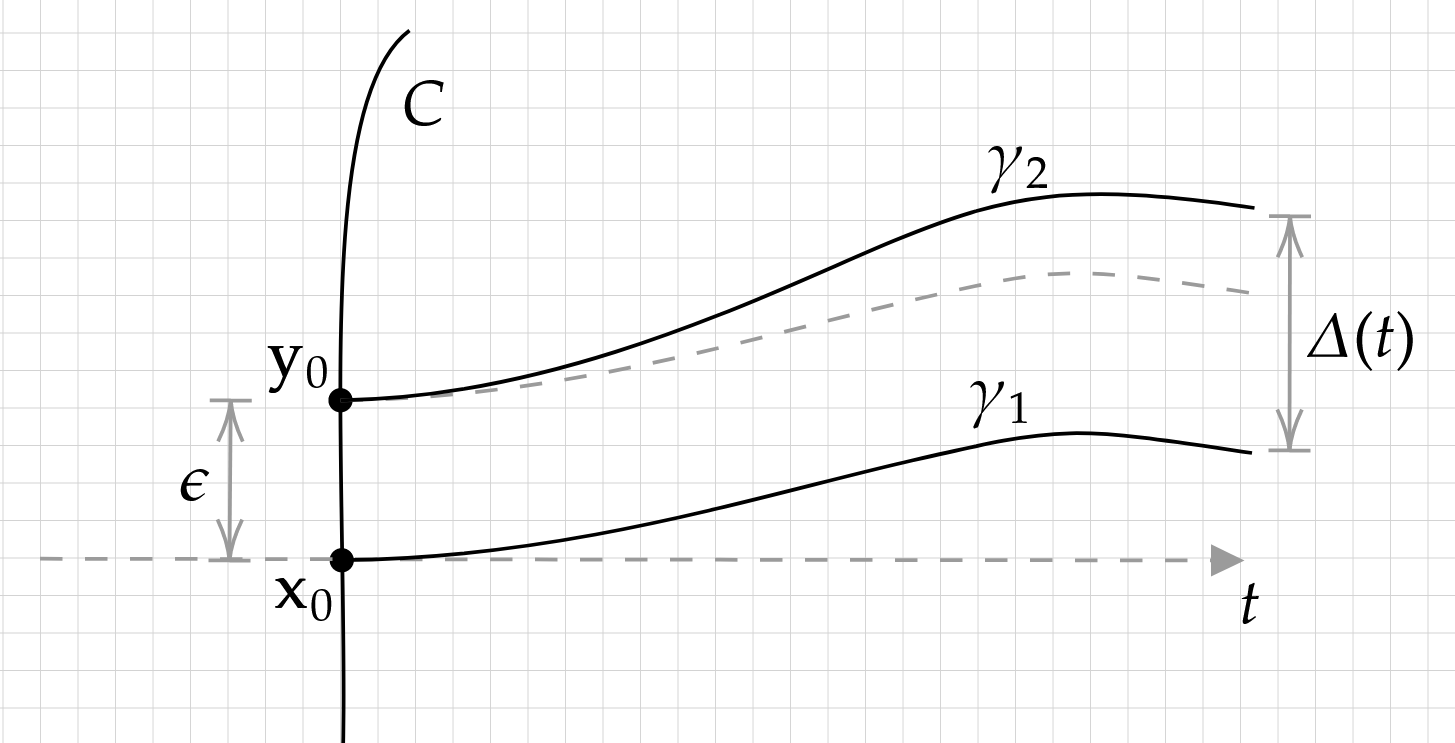
If \(f\) is locally Lipschitz, then so is \(\tilde{f}=f_y/f_x\) for small enough \(W\). For notational convenience — since it doesn't matter what the Lipschitz constant actually is — we'll also say that \(\tilde{f}\) has Lipschitz constant \(K\). As previously established in the proof of Picard's Existence Theorem, we can use the streamline differential equation \(\gamma_1'(t)=\tilde{f}(t,\gamma_1(t))\) to generate the streamline passing through \(\mathbf{x}_0\), provided that \(\gamma_1(0)=0\). The streamline \(\gamma_2\) passing though \(\mathbf{y}_0\) likewise follows \(\gamma_2'(t)=\tilde{f}(t,\gamma_2(t))\), where \(\gamma_2(0)=\epsilon\).
We're looking to bound the deviation of \(\gamma_2\) from \(\gamma_1\) in terms of \(\epsilon\). We know that \(\tilde{f}\) is Lipschitz, so we can write \[ \begin{align*} |\gamma_2'(t)-\gamma_1'(t)|&= | f(t,\gamma_2(t)) - f(t, \gamma_1(t)) | \\ &\leq K|\gamma_2(t)-\gamma_1(t) |\,. \end{align*} \] Without loss of generality, we can assume that \(\epsilon \geq 0\) so that \(\gamma_2 \geq \gamma_1\), noting that streamlines cannot cross each other. Moreover, the error \(\Delta(t)\) is maximized when \(\gamma_2'\) is maximized. According to our inequality above, then, \(\gamma_2\) is less than or equal to the solution to the ODE \[ \gamma_2'(t)-\gamma_1'(t)=K(\gamma_2(t)-\gamma_1(t)) \iff (\gamma_2-\gamma_1)'(t)=K(\gamma_2-\gamma_1)(t) \,, \] i.e. \(|\Delta(t)| \leq \epsilon \cdot e^{K t}\). The maximal \(t\) is a geometric quantity based on the diameter of \(W\), a fixed quantity. Then we can say \(|\Delta(t)|\leq \epsilon\cdot e^{KR}\) for some fixed \(R\). Now by shrinking \(W\) so that \(f\) varies little, we can ensure that the \(\nu\)-measure of the contour between \(\mathbf{x}_0\) and \(\mathbf{y}_0\) is comparable with \(\epsilon\), say by a constant scaling factor. Indeed, the area between the contours \(\gamma_1\) and \(\gamma_2\) is proportional to \(\epsilon\) (it would go something like \(R\epsilon\cdot e^{KR}\)).
We are finally ready to tackle the theorem. Suppose that \(A\subset C\) is a set with \(\nu\)-measure zero. Since \(\nu\) is regular (it's a finite measure on a metric space), there is a finite set of intervals \(\{I_j\}_j\) that cover \(A\) so that \(\sum_j \nu(I_j)\leq \epsilon\) for any \(\epsilon > 0\). By "interval", we mean \(\lambda([a,b])\) for some \(a,b\in \mathbb{R}\), where \(\lambda\) is the contour streamline passing through \(\mathbf{x}_0\). We just found that \(G(I_j)\leq M \nu(I_j)\) for some constant \(M\), so we immediately see that \[ G\left(\bigcup_i I_j\right)\leq \sum_j G(I_j) \leq M\sum_j \nu(I_j) \leq M\epsilon\,. \] Since \(\epsilon\) is arbitrary, it must be that \(G(A)=0\). (QED)
The Local Equation for \(g\)
It's important to remember that \(g\) is defined up to \(L^1(C, d\nu)\) equivalence, i.e., \(g\) is only unique up to a set of \(\nu\)-measure zero on a contour \(C\). However, we can secretly guess that \(g\) is supposed to be continuous, and indeed the Lebesgue Differentiation Theorem gives us a handy way to produce a candidate. Let \[ \tilde{g}(\mathbf{x}):=\lim_{I \to \mathbf{x}}\frac{1}{\nu(I)}\int_I g\,. \] The neighborhood \(I\) is shorthand for an interval on the contour \(C\). If the contour is the image \(\lambda([a,b])\) for some contour streamline \(\lambda\), then \(I\) can be written \(I=\lambda([\lambda^{-1}(\mathbf{x})-\delta, \lambda^{-1}(\mathbf{x})+\delta])\), with \(I\to \mathbf{x}\) indicating \(\delta\to 0\). That \(\tilde{g}\) is \(\nu\)-almost-everywhere equal to \(g\) is a consequence of a slightly strengthened version of the Lebesgue Differentiation Theorem quoted above (which only deals with Lebesgue measures), but since \(\nu\) is so nice it is straightforward; see here for example.
Armed with a pointwise representative \(\tilde{g}\) of \(g\), we can tackle continuity directly. Let \(\mathbf{x}\) and \(\mathbf{y}\) be two points on a contour \(C\). \(\tilde{g}\) is continuous on \(C\) if \(\lim_{\mathbf{x}\to\mathbf{y}} |\tilde{g}(\mathbf{x})-\tilde{g}(\mathbf{y})|=0\,. \) We calculate \[ \begin{align*} \lim_{\mathbf{x}\to\mathbf{y}} |\tilde{g}(\mathbf{x})-\tilde{g}(\mathbf{y})|&= \lim_{\mathbf{x}\to\mathbf{y}}\left| \lim_{I_1\to\mathbf{x}} \frac{G(I_1)}{\nu(I_1)} - \lim_{I_2\to\mathbf{y}}\frac{G(I_2)}{\nu(I_2)} \right| \\ &= \lim_{\mathbf{x}\to\mathbf{y}}\left| \lim_{r\to 0}\frac{1}{2r}\left( G(C\cap(\mathbf{x}+B_r)) - G(C\cap(\mathbf{y}+B_r)) \right) \right| \\ &\leq \lim_{\mathbf{x}\to\mathbf{y}} \lim_{r\to 0} \frac{1}{2r}G(C \cap ((\mathbf{x}+B_r) \bigtriangleup (\mathbf{y}+B_r))) \\ &\leq \lim_{r\to 0} \lim_{\mathbf{x}\to\mathbf{y}}\frac{1}{2r}G(C \cap ((\mathbf{x}+B_r) \bigtriangleup (\mathbf{y}+B_r))) \\ &\leq \lim_{r\to 0} \frac{1}{2r}\lim_{\mathbf{x}\to\mathbf{y}} 2K|\mathbf{x}-\mathbf{y}| \\ &= 0\,. \end{align*} \] There's a bit going on here. We immediately make the substitution \(\int_I g=G(I)\), as per the definition of \(g\). The set \(B_r=\{\mathbf{z}\in \mathbb{R}^2 : |\mathbf{z}|\leq r\}\) provides a convenient way to write \(I_1\) and \(I_2\) in terms of a common variable \(r\). Although \(\nu(I_1)\) and \(\nu(I_2)\) vary slightly from \(\frac{1}{2r}\), since contours are differentiable this is an accurate approximation when \(\mathbf{x}\to \mathbf{y}\), and the multiplicative constants aren't relevant here. The symbol "\(\bigtriangleup\)" is used as the set symmetric difference, noting that \(G\) is a positive measure. The limit rearranging is justified by restricting \(W\) to some small neighborhood of \(\mathbf{x}\) and \(\mathbf{y}\), in which case \( |\tilde{g}(\mathbf{x})| \) and \(|\tilde{g}(\mathbf{y})|\) are bounded by the estimate \(G(I)\leq M\nu(I)\) generated in the previous section. Then a cheeky application of the dominated convergence theorem suffices to switch the limit order. The \(K|\mathbf{x}-\mathbf{y}|\) term likewise comes from the estimate \(G(I)\leq M\nu(I)\).
From here on, when we write "\(g\)", we really mean the pointwise-defined, continuous representative \(\tilde{g}\).
Since every point \(\mathbf{x}\in W\) belongs to a unique contour, \(g\) extends without ambiguity to all of \(W\). Moreover, since \(g\) is continuous on contours with \( \left|\int_{\lambda_1}g - \int_{\lambda_2}g\right| \) equal to the area between \(\lambda_1\) and \(\lambda_2\) (more or less), it is not difficult to show that \(g\) is continuous on all of \(W\) (a fun exercise for the reader, perhaps).
Proof: Pick a point \(\mathbf{x}\) in \(W\), and let \(U\subset W\) be a neighborhood of \(\mathbf{x}\). Make \(U\) small enough so that contours and streamlines around \(\mathbf{x}\) are roughly straight, and consider the following figure:
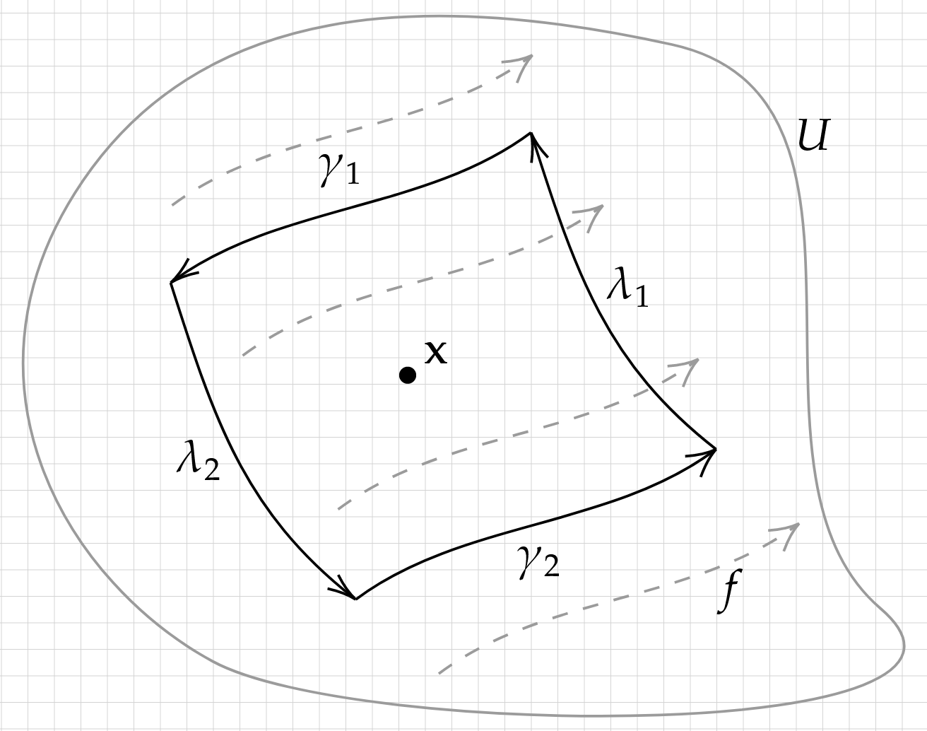
Here \(\gamma_1\) and \(\gamma_2\) are streamlines (with \(\gamma_1\) the wrong direction); \(\lambda_1\) and \(\lambda_2\) are contour streamlines. Consider the loop \(\Gamma\), the concatenation of \(\lambda_1\), \(\gamma_1\), \(\lambda_2\) and \(\gamma_2\), in counter-clockwise order. The expression in question will be \[ \int_\Gamma g (f_x dy - f_y dx)\,. \] On the streamlines \(\gamma_1\) and \(\gamma_2\), \(f_x dy - f_y dx\) vanishes. On \(\lambda_1\), \(f\) is orthogonal to \(\lambda_1'\) and correctly oriented, so that \(\int_{\lambda_1}g(f_x dy-f_ydx)=G(\lambda_1)\). On \(\lambda_2\), \(f\) is orthogonal to \(\lambda_2'\) but incorrectly oriented, so that \( \int_{\lambda_2}g(f_xdy-f_ydx)=-G(\lambda_2) \). The upshot is that \[ \int_\Gamma g (f_x dy - f_y dx) = G(\lambda_1) - G(\lambda_2)\,. \] This is nothing but the area of the region \(\Gamma^\mathrm{o}\) enclosed by \(\Gamma\), i.e., \(\int_{\Gamma^\mathrm{o}} dx\wedge dy\). On the other hand, we can apply Stoke's theorem to the left side \(\int_\Gamma g (f_x dy - f_y dx)\), obtaining \[ \begin{align*} \int_\Gamma g (f_x dy - f_y dx) &= \int_{\Gamma^\mathrm{o}} \partial \left( g f_x dy - g f_y dx \right) \\ &= \int_{\Gamma^\mathrm{o}} \partial (g f_x) \wedge dy - \partial(g f_y) \wedge dx \\ &= \int_{\Gamma^\mathrm{o}} \frac{d}{dx}(g f_x) \wedge dy - \frac{d}{dy} (g f_y) \wedge dx \\ &= \int_{\Gamma^\mathrm{o}} \left( g\left(\frac{df_x}{dx} + \frac{df_y}{dy}\right) + f_x \frac{dg}{dx} + f_y \frac{dg}{dy} \right) dx \wedge dy \\ &= \int_{\Gamma^\mathrm{o}} \left( (\nabla \cdot f)g + \nabla g \cdot f \right) dx \wedge dy\,. \end{align*} \] In the limit where \(\Gamma^{\mathrm{o}}\) becomes small, since \((\nabla \cdot f)g + \nabla g \cdot f\) is continuous, we have \[ \int_{\Gamma^\mathrm{o}} \left( (\nabla \cdot f)g + \nabla g \cdot f \right) dx \wedge dy = \int_{\Gamma^\mathrm{o}} dx\wedge dy \implies (\nabla \cdot f)g + \nabla g \cdot f = 1\,. \] (QED)